Color scales based on Gavi color palette

Usage

scale_color_gavi(palette = "standard", discrete = TRUE, reverse = FALSE, ...)

Arguments

palette: A palette. Defaults to standard palette, but other palettes also available. Full list: all, standard, millennial, main, strategy, vaccine, who_region, gavi_segment, world_bank, red_green, traffic, misc1, misc2, map_blue_red, map_blue_red2, map_orange_turquoise, map_green_red, map_blues, map_reds, map_greens.
discrete: Defaults to TRUE, keep if data is discrete. If continuous, used FALSE.
reverse: Reverses order of palette.
...: Additional arguments passed to ggplot2::discrete_scale() or ggplot2::scale_fill_gradientn(), used respectively when discrete is TRUE or FALSE

Examples

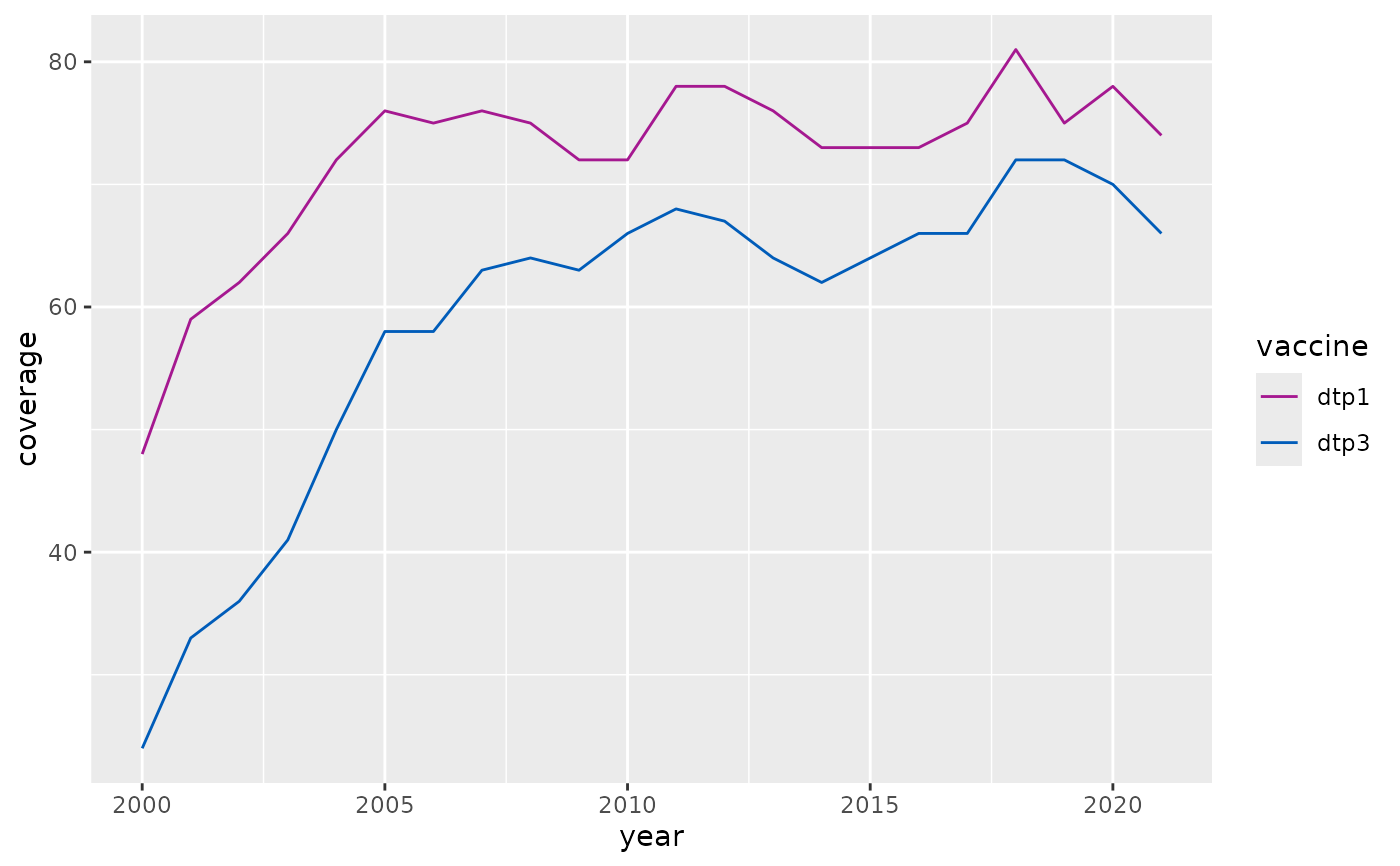
# Example one - applied to discrete data
library(dplyr)
library(ggplot2)
wuenic %>%
 filter(iso3 == "AFG" & vaccine %in% c("dtp1", "dtp3")) %>%
 ggplot(aes(year, coverage, color = vaccine)) +
 geom_line() +
 scale_color_gavi()


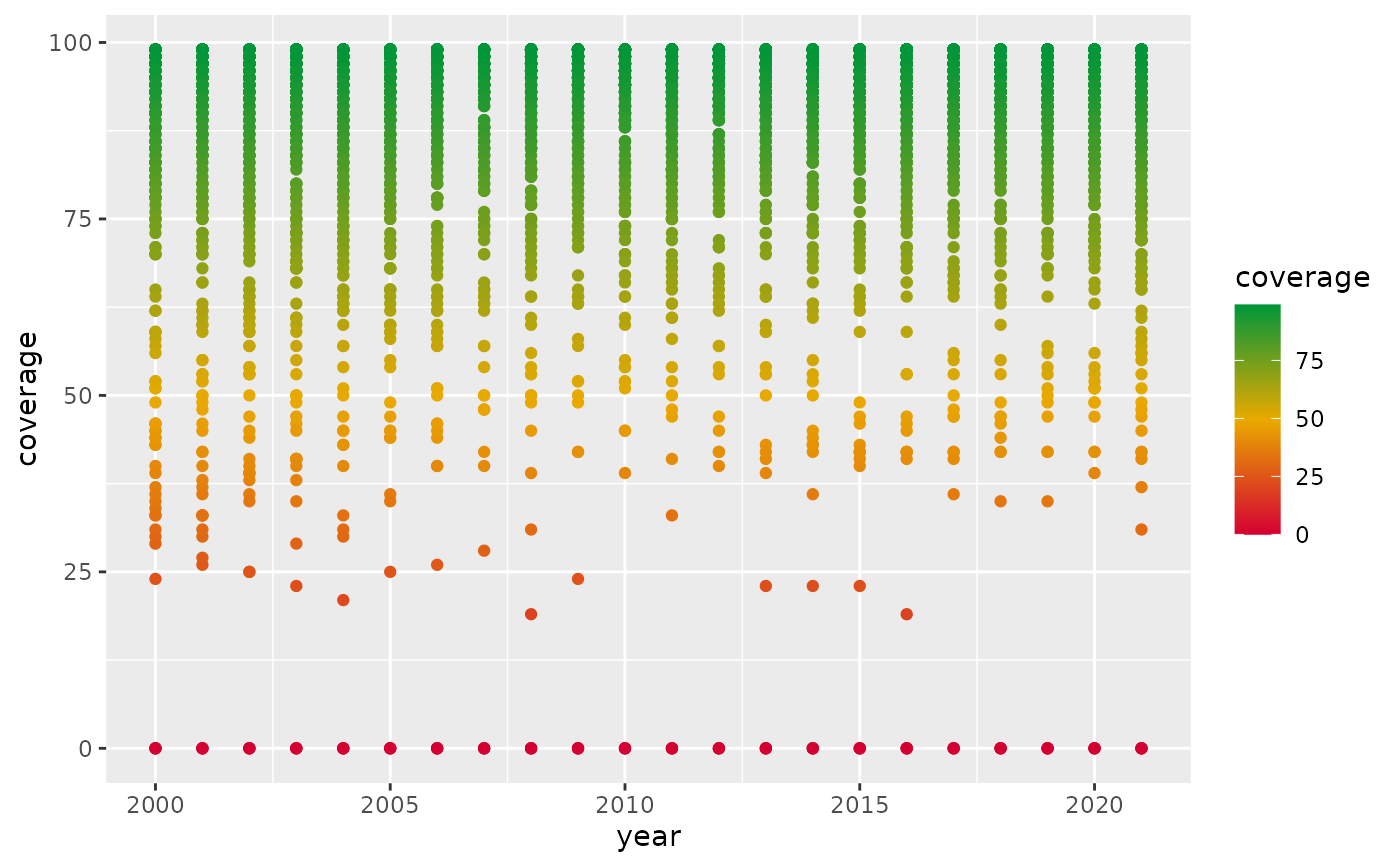
# Example two - with different palette, and continuous data
wuenic %>%
 filter(vaccine == "dtp3" & !is.na(coverage)) %>%
 ggplot(aes(year, coverage, color = coverage)) +
 geom_point() +
 scale_color_gavi(palette = "traffic", discrete = FALSE)